If you have worked with MS Excel for a while I bet you have had the need to highlight/count unique or duplicate values. In this post I’ll cover all you need to know to deal with duplicate/unique values in MS Excel.
After reading this post you’ll be able to:
- Highlight duplicate values in MS Excel
- Highlight duplicate values starting at the second occurrence of each value
- Highlight unique values
- Highlight the first occurrence of each value
- Count unique values using formulas
- Remove duplicate values from a dataset
- Count distinct values in PivotTables
How to Highlight Duplicates in MS Excel
Finding duplicates in existing data is one of the important features of MS Excel. You can do it with just a few clicks through the ‘Conditional Formatting’ menu option.
The ‘Conditional Formatting’ menu option can be found on the Home tab of Excel 2013 as shown below.
Figure 1: Conditional Formatting Option
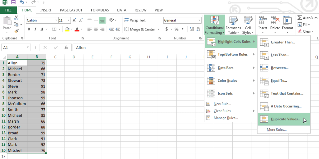
Now if we have the duplicate values in a column or columns (as we have in columns A and B in figure2 below), the following steps can be carried out to highlight the duplicate values.
- Select the required range (i.e. columns A and B in our case).
- Click on ‘Conditional Formatting‘ ‘Highlight Cells Rules‘ ‘Duplicate Values‘.
Figure 2: Steps to highlight duplicate values
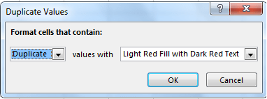
- You will see a window as shown below, Click “OK“.
Figure 3: Format cells window
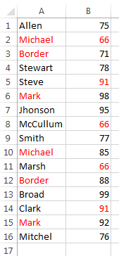
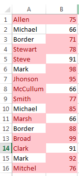
You will see that duplicate values are highlighted as shown below:
Figure 4: Highlighted duplicate values
How to highlight cell rules after second occurrence
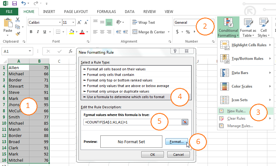
If you use the steps shown above, you’ll be able to highlight ALL the occurrences of the values with duplicates. However, sometimes we want to highlight the second occurrence or later occurrences of the duplicate values. This can be accomplished by following the next steps:
- Select the range with duplicate values (i.e. range A1:B16 in our case).
- Go to ‘Home’ ‘Conditional Formatting‘.
- Click on ‘New Rule‘.
- Click on ‘Use a formula to determine which cells to format‘.
- Type ‘=COUNTIF($A$1:A1,A1)>1‘ in formula bar. The general pattern for the formula is =COUNTIF(first cell of range locked with dollar signs : first cell of range unlocked, first cell of range unlocked) > 1
- Click on the ‘Format‘ button.
- Change the format as desired for duplicate values, you can change the format for Numbers, Font, Borders, and Fill.
- Click ‘OK‘.
- Click ‘OK‘ again.
Steps are shown below for your convenience.
Figure 1: Steps to highlight the values after the second occurrence
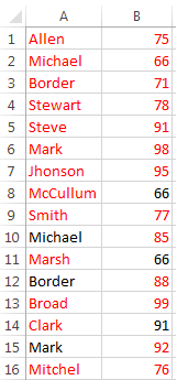
You will see that duplicate values are highlighted after the second occurrence as shown in figure 2 below.
Figure 2: Highlighted values after the second occurrence
How to highlight unique values
If you read the first section, you already know how to highlight duplicates in Excel. You can follow almost the same steps to highlight unique values in a range. By unique values I mean values that only appear once in a range.
Follow these steps to highlight unique values in a range:
- Select the required range.
- Click on ‘Conditional Formatting‘ ‘Highlight Cells Rules‘ ‘Duplicate Values‘.
- You will see a window shown in Figure 1 below.
Figure 1: Duplicate Values
The default option selected is ‘Duplicate‘. Click on the down arrow and select ‘Unique‘ as shown in figure 2 below.
Figure 2: Unique Values Option
You will see that the unique values in the selected range are highlighted as shown in figure 3 below.
Figure 3: Highlighted Unique Values
How to Highlight the First Occurrence of Each Value
Instead of highlighting only the values that appear once in the range, sometimes we want to highlight only the first occurrence of each value. To do this, follow these steps:
- Select the range with the duplicate values (i.e. in our case the range A1:B16)
- Click on ‘Conditional Formatting‘.
- Click on ‘New Rule‘.
- Click on ‘Use a formula to determine which cells to format‘.
- Type ‘=COUNTIF($A$1:A1,A1)=1‘ in the formula bar. The general pattern for the formula is =COUNTIF(first cell of range locked with dollar signs : first cell of range unlocked, first cell of range unlocked) = 1
- Click on ‘Format‘ button.
- Select a color of your choice.
- Click ‘OK‘ button.
- Click ‘OK‘ button again.
Figure 1: Steps to highlight the first occurrence of each value
You will see that the values are highlighted at the first occurrence as shown below.
Figure 2: Highlighted values at the first occurrence
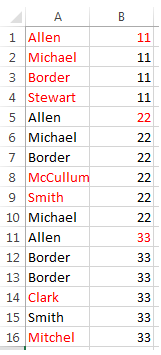
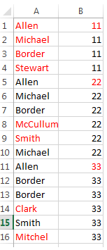
The following figure shows another example to highlight the first occurrence of each value.
Figure 3: Another example of highlighted values at the first occurrence
How to Count Unique Values
A very important feature of Excel is that you can count the number of unique values in a given range. This task can be done in at least two ways. We will discuss both ways in this tutorial.
Method #1: Simple formula
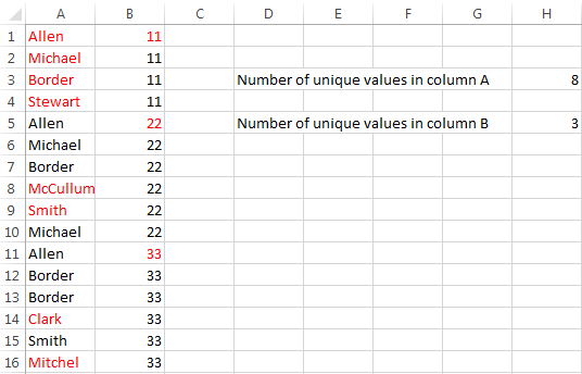
The first method to count the unique values is by combining SUMPRODUCT() and COUNTIF() functions. Consider the values given in figure 1 below. I have already highlighted the unique values for the convenience. We can count the unique values by writing the following formulas in cell H3 and H5 respectively.
=SUMPRODUCT(1/COUNTIF(A1:A16,A1:A16))
=SUMPRODUCT(1/COUNTIF(B1:B16,B1:B16))
The general pattern is:
=SUMPRODUCT(1/COUNTIF(Range, Range))
The result of these formulas is shown in figure 2 below.
Figure 1: Sample data
Figure 2: Number of unique values
The formula shown above is the simplest way of counting unique values. However, you might encounter some scenarios where you might need to tweak it a little bit. For example, if there are empty cells in the range you can do this:
=SUMPRODUCT((Range <> “”)/(COUNTIF(Range, Range&””))
Method #2: Complex and Robust formula
The method mentioned above is useful when you need to quickly count the number of unique values in a small range. However, for more complex scenarios such as large ranges (lots of cells), lots of empty spaces, it is better to use a more robust and efficient formula.
The formula recommended to count unique values in a Range for this complex cases is:
=SUMPRODUCT(IF(FREQUENCY(MATCH(Range, Range, 0), MATCH(Range, Range, 0)) > 0, 1))
For our specific example, the ranges where we want to count unique values are: A1:A16 and B1:B16; therefore the formulas would be:
=SUMPRODUCT(IF(FREQUENCY(MATCH(A1:A16, A1:A16,0),MATCH(A1:A16, A1:A16, 0))>0,1))
=SUMPRODUCT(IF(FREQUENCY(MATCH(B1:B16, B1:B16,0),MATCH(B1:B16, B1:B16, 0))>0,1))
The result of these formulas will be same as shown in figure 2 above.
How to Remove Duplicates
Sometimes we want to remove the duplicate values from a range.
Fortunately, MS Excel has a feature to do exactly that, remove duplicate values in a range according to the values in one or several columns.
Consider the values in the following sheet (I have already highlighted the duplicate values for convenience):
Figure 1: Sample data having duplicate values
We can follow the following steps to remove the duplicate values.
- Select the required cell range i.e. A1:A16 in our example.
- Click the ‘Data‘ tab.
- Click on ‘Remove Duplicates‘ option as shown in figure 2 below.
Figure 2: Remove duplicates option
- You will be asked to select the column(s) where duplicates will be removed i.e. Column A in our case.
- Click ‘OK‘.
- You will be notified about the number of duplicate and unique values as shown in the figure below
Figure 2: Duplicate and unique values notification
After removing the duplicates, you will get a list of values having unique values only as shown below.
Figure 3: List of unique values after removing duplicates
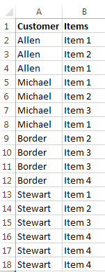
Notice that you can remove the duplicate values by considering several columns at the same time. For example, let’s say we want to remove the duplicates values from columns A and B in the next range:
Figure 4: Multiple columns for remove duplicates
Just repeat the same steps:
- Select range, i.e., range A1:B18
- Go to Data Remove duplicates
- In the checkbox that will appear, select the column titles you want to consider for the duplicates elimination. Notice that you will ONLY select the column titles for the columns where the duplicates will be considered, regardless of the number of columns in the data range.
Figure 5. Columns selection for remove duplicates
- Click OK
How to count distinct values in PivotTables using the Excel Data Model in 2013
Probably one of the most awaited PivotTable features in native Excel was the ability to count distinct values. Fortunately, starting on Excel 2013 Microsoft introduced the capability of counting distinct values in PivotTables without using complex tricks.
Before exploring this feature, let us see what was the problem with pivot tables.
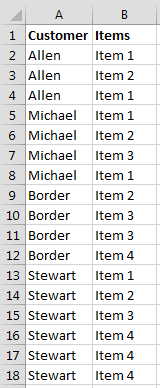
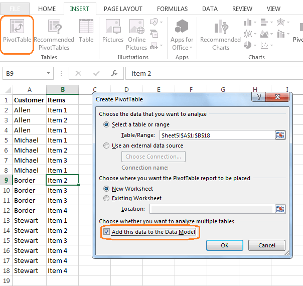
Suppose we have data about customers and their orders. Different customers have ordered different items as shown in the figure below.
Figure 1: Sample data
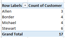
If we are interested to find the number of distinct items ordered by each customer, then we can create a pivot table by following the steps given below but normal pivot table cannot satisfy our requirement. Normal pivot table just counts the number of items against each customer rather than providing the distinct count of items.
- Click on anywhere in the range.
- Click on ‘INSERT‘ tab.
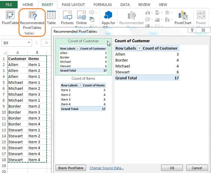
- Click on ‘Recommended Pivot Tables‘ ‘Count of Customer‘ ‘OK‘
Figure 2: Steps to create pivot table
You will get a pivot table as shown below. You can clearly see that it counts the TOTAL number of items against each customer while we are interested to count the DISTINCT number of items ordered by each customer. ‘Allen’ ordered Item1, Item2, Item1 so the count is 3 as shown but the distinct count is 2 (Item1 and Item2).
Figure 3: Pivot table showing the total number of counts
In order to solve this issue, you can use the data model feature in MS Excel 2013 or later by following the next steps:
- Click anywhere in the range.
- Click on ‘INSERT‘ tab.
- Click on ‘Pivot Table‘.
- Click on ‘Add this data to the Data Model‘ checkbox. It MUST be checked to get the desired result.
- Click ‘OK‘
Figure 4: Excel 2013 pivot table
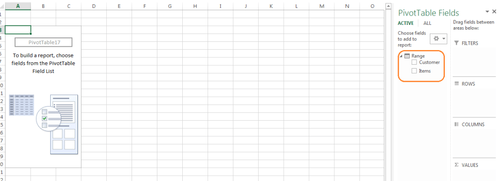
- When you click OK, MS Excel 2013 will add your data to the data model. After clicking ‘OK’, you will get a screen as below. Drag the ‘Customer’ field to the ROWS area and the ‘Items’ Field to the VALUES area.
Figure 5: Excel 2013 pivot table options
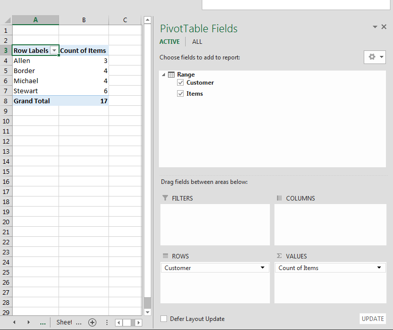
After moving the fields, the PivotTable will look like this.
Figure 6: Pivot table showing customers and items
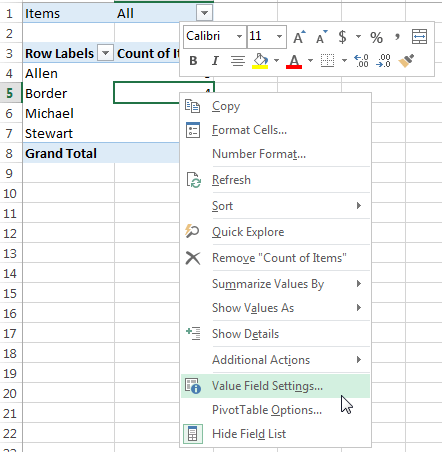
- Right click on any item in second column.
- Click on ‘Value Field Settings…‘.
Figure 8: Value Field Settings
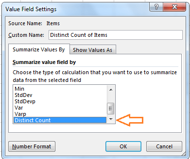
- After clicking on ‘Value Field Settings…‘, you will get a screen as below. Select the ‘Distinct Count‘ option.
- Click on ‘OK‘.
Figure 9: Distinct count option
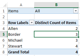
After clicking ‘OK‘, you will see what was desired: a distinct count of items for every customer.
Figure 10: Distinct count of values
As you can see, there a many tips to deal with duplicates in Excel. Do you know more? Please post them in the comments section!
Please share this post so more people can benefit!
© Master Data Analysis All Rights Reserved 2024


